---
title: "It takes 242,516 minutes to do a PhD"
date: "2025-04-16"
categories: [PhD]
image: "imgs/proj-hrs.png"
toc: true
format:
html:
code-fold: true
code-tools: true
---
That's 4041 hours and 56 minutes!
I tracked all my work time during the PhD, and now that it's done, I can finally crunch the numbers.
# The data
```{r setup, message = FALSE}
library(tidyverse)
library(patchwork)

theme_set(theme_bw())
theme_update(
  text = element_text(family = "Fira Sans", size = 12),
  panel.grid = element_blank(),
  strip.background = element_blank(),
  axis.title.y = element_text(angle = 0, vjust = 0.5, hjust = 0)
)

palette_year <- c("#51b375", "#ff94b0", "#1c4a86", "#ed7a1d")
palette_tasktype <- c("#1c4a86","#51b375", "#FFCD29", "#3173c9", "#bb3725")
palette_proj <- c("#bb3725", "#FFCD29","#51b375", "#3173c9")
palette_exam <- c("#1c4a86", "#bb3725")

# Read in the data and display first few rows.
hrs <- read_csv('data/hrs.csv') |>
  mutate(
    year_idx  = factor(year_idx),
    year      = factor(year)
  )
head(hrs) |>
  knitr::kable()
```
This dataset contains only the time I spent on core PhD tasks.
All my non-PhD collaborations and side projects have been filtered out.
```{r}
#| code-fold: false
sum(hrs$mins)
```
From attending my first reading group on September 9, 2021, to submitting my thesis corrections on April 9, 2025, I worked on the PhD for 242,516 minutes.
(And if reading that makes the song from RENT start playing in your head, you are not alone 🙈)
# How many hours per day?
```{r message = FALSE}
year_labs <- tibble(
  date = c(
    as.Date('28/02/2022', "%d/%m/%Y"),
    as.Date('28/02/2023', "%d/%m/%Y"),
    as.Date('28/02/2024', "%d/%m/%Y"),
    as.Date('31/12/2024', "%d/%m/%Y")
    ),
  daily_hrs = 13.5,
  lab = paste('Year', 1:4),
  year_idx = factor(1:4)
)

hrs_daily <- hrs |>
  group_by(date, year_idx) |>
  summarise(
    daily_hrs = sum(mins)/60,
  )

p_daily_point <- hrs_daily |>
  ggplot(aes(x = date, y = daily_hrs, colour = year_idx)) +
  geom_point(alpha = 0.5) +
  geom_smooth(method = 'lm', se = FALSE, linewidth = 2) +
  geom_text(data = year_labs, aes(label = lab), family = 'Fira Sans', size = 4) +
  labs(
    y = 'Hours/\nday',
    x = element_blank(),
    colour = 'Year of the PhD'
  ) +
  theme(legend.position = 'none') +
  scale_colour_manual(values = palette_year) +
  scale_y_continuous(breaks = seq(0, 12, 3), limits = c(0, 14)) +
  NULL

p_daily_violin <- hrs_daily |>
  ggplot(aes(x = year_idx, y = daily_hrs, colour = year_idx, fill = year_idx)) +
  geom_violin(alpha = 0.5) +
  geom_jitter(alpha = 0.5, width = 0.1) +
  scale_fill_manual(values = palette_year) +
  scale_colour_manual(values = palette_year) +
  scale_x_discrete(labels = paste('Year', 1:4)) +
  theme(legend.position = 'none') +
  labs(
    y = 'Hours/\nday',
    x = element_blank()
  ) +
  NULL

p_daily_point / p_daily_violin
```
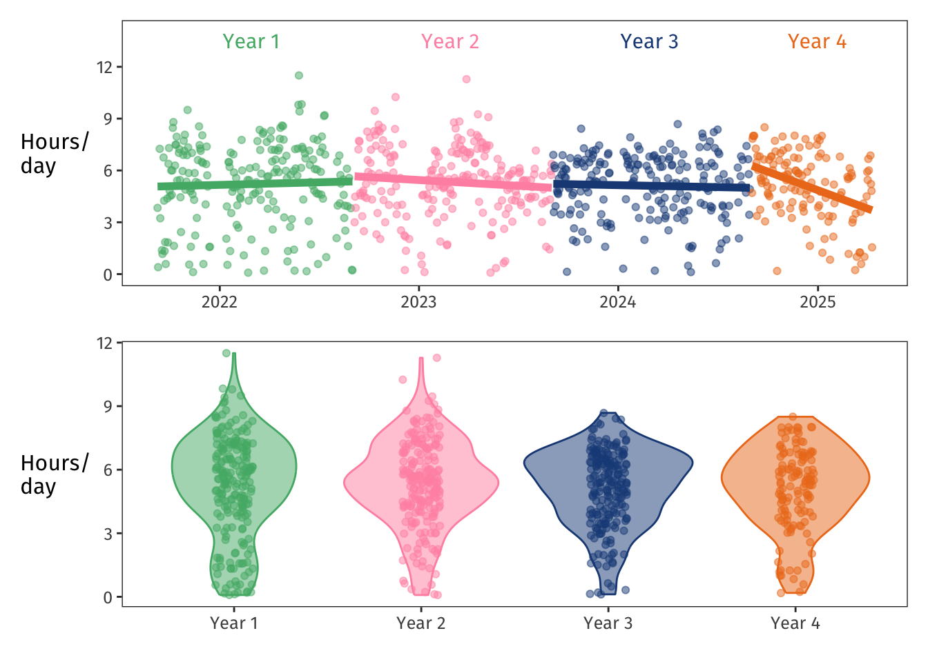
The upper plot shows that as **Year 1** (green) went on, my time spent on PhD things slightly increased—makes sense, since I was wrapping up other lingering projects and turning my focus more and more to the PhD.
**Year 2** (pink) shows a slight a drop-off over time.
Then **Year 3** (blue) was pretty stable, and **Year 4** (orange) started with some vigorous experiment-running and thesis-writing, then decreased quickly as the PhD reached an end.
The violins in the lower plot aggregate the data for each year.
They show that in Years 1 and 2, I worked too long too often—I'm glad I got that impulse under control for Years 3 and 4.
```{r message = FALSE}
hrs_daily |>
  ungroup() |>
  summarise(
    mean_daily   = round(mean(daily_hrs), 1),
    median_daily = round(median(daily_hrs), 1),
    min_daily    = round(min(daily_hrs), 2),
    max_daily    = round(max(daily_hrs), 1)
  ) |>
  knitr::kable()
```
Overall, on average I spent 5.2 hours per day focused on PhD work.
My median work day was 5.4 hours.
My shortest work day was five minutes (lol), and my longest work day was 11.5 hours (bad. don't do this).
# How many hours per task type?
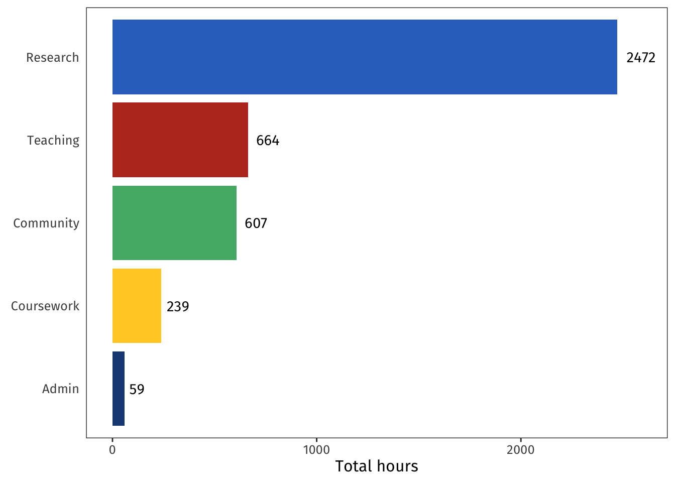
My work fell into five broad categories:
- **Admin:** Covers misc set-up and bureaucracy around the PhD, as well as my admin tasks within my research group.
- **Community:** Covers reading groups, talk series, and conferences/workshops.
- **Coursework:** Covers the required courses that were a condition of my funding as well as courses I audited for fun.
- **Research:** Covers reading the literature, designing and implementing experiments and models, writing everything up, preparing talks, and the PhD examination process.
- **Teaching:** Covers tutoring, guest lecturing, my one-on-one stats chats sessions, and working toward my AFHEA accreditation.
```{r}
hrs |>
  group_by(tasktype) |>
  summarise(hrs = sum(mins)/60) |>
  arrange(hrs) |>
  mutate(tasktype = factor(tasktype, levels = tasktype)) %>%
  ggplot(aes(y = tasktype, x = hrs, fill = tasktype)) +
  geom_col() +
  geom_text(
    aes(
      label = round(hrs),
      x = hrs + (15 * log(hrs))  # scale the spacing by magnitude of hrs
    ), family = 'Fira Sans') +
  labs(
    y = element_blank(),
    x = 'Total hours'
  ) +
  theme(
    axis.ticks.y = element_blank(),
    legend.position = 'none'
  ) +
  scale_fill_manual(values = c(palette_tasktype[1], palette_tasktype[3], palette_tasktype[2], palette_tasktype[5], palette_tasktype[4]))+
  NULL
```
This looks about right!
Lots and lots of research, plenty of teaching and community engagement, a bit of course work, with admin sitting blissfully in last place.
# Task types over time
```{r message = FALSE}
hrs |>
  group_by(month_idx, tasktype, year) |>
  summarise(hrs = sum(mins)/60) |>
  ggplot(aes(x = month_idx, y = hrs, fill = tasktype)) +
  geom_bar(stat = 'identity', position = 'stack') +
  scale_x_continuous(breaks = c(5, 17, 29, 41), labels = c(2022, 2023, 2024, 2025)) +
  labs(
    y = 'Hours/\nmonth',
    x = element_blank(),
    fill = element_blank()
  ) +
  scale_fill_manual(values = palette_tasktype) +
  NULL
```
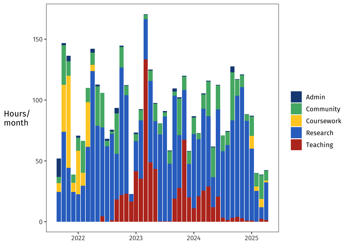
I did a lot of tasks pretty regularly across the whole four years: regular admin, regular community engagement, regular research.
The big swaths of yellow coursework in the beginning were my required courses, and the for-fun auditing happened toward the end.
The big red spike of teaching in early 2023 is when I stepped in to design and run the last several weeks of a PG-level Bayesian stats course.
That was such a fun and formative experience—it's hard to believe that it was more than half a PhD ago.
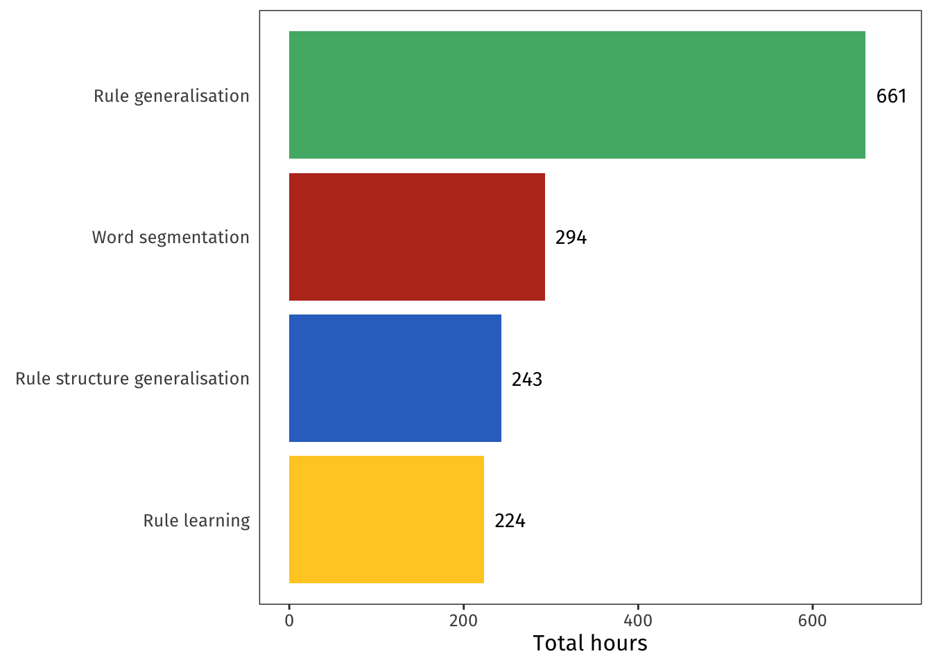
# How many hours per research project?
I conducted four research projects during the PhD, and each project makes up one content chapter in my thesis.
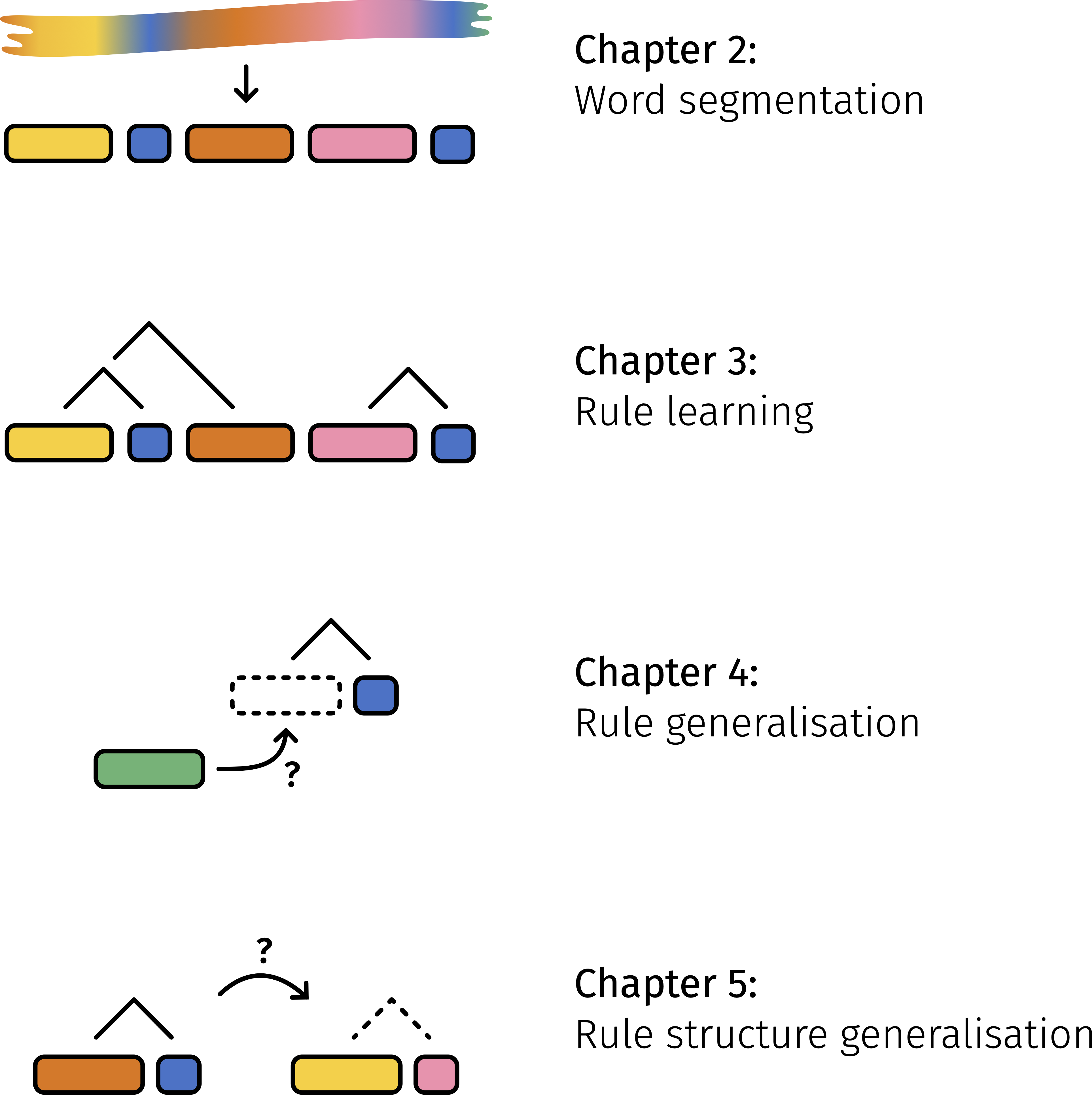{width=60% fig-align="center"}
My time on these projects was lumped together under the **Research** task type I plotted above, but of course I also recorded how much time I spent on each project individually.
```{r}
main_projs <- c('Word segmentation', 'Rule learning',  'Rule generalisation',  'Rule structure generalisation')

hrs |>
  filter(tasklabel %in% main_projs) |>
  group_by(tasklabel) |>
  summarise(hrs = sum(mins)/60) |>
  arrange(hrs) |>
  mutate(tasklabel = factor(tasklabel, levels = tasklabel)) |>
  ggplot(aes(y = tasklabel, x = hrs, fill = tasklabel)) +
  geom_col() +
  geom_text(
    aes(
      label = round(hrs),
      x = hrs + 30
    ), family = 'Fira Sans') +
  labs(
    y = element_blank(),
    x = 'Total hours'
  ) +
  theme(
    axis.ticks.y = element_blank(),
    legend.position = 'none'
    ) +
  scale_fill_manual(values = c(palette_proj[2], palette_proj[4], palette_proj[1], palette_proj[3])) +
  NULL
```
I always knew that the **Rule generalisation** project (green, Chapter 4) was closest to my heart, but I'm still amused to see that I dedicated more than double as much time to it as to any of the others.
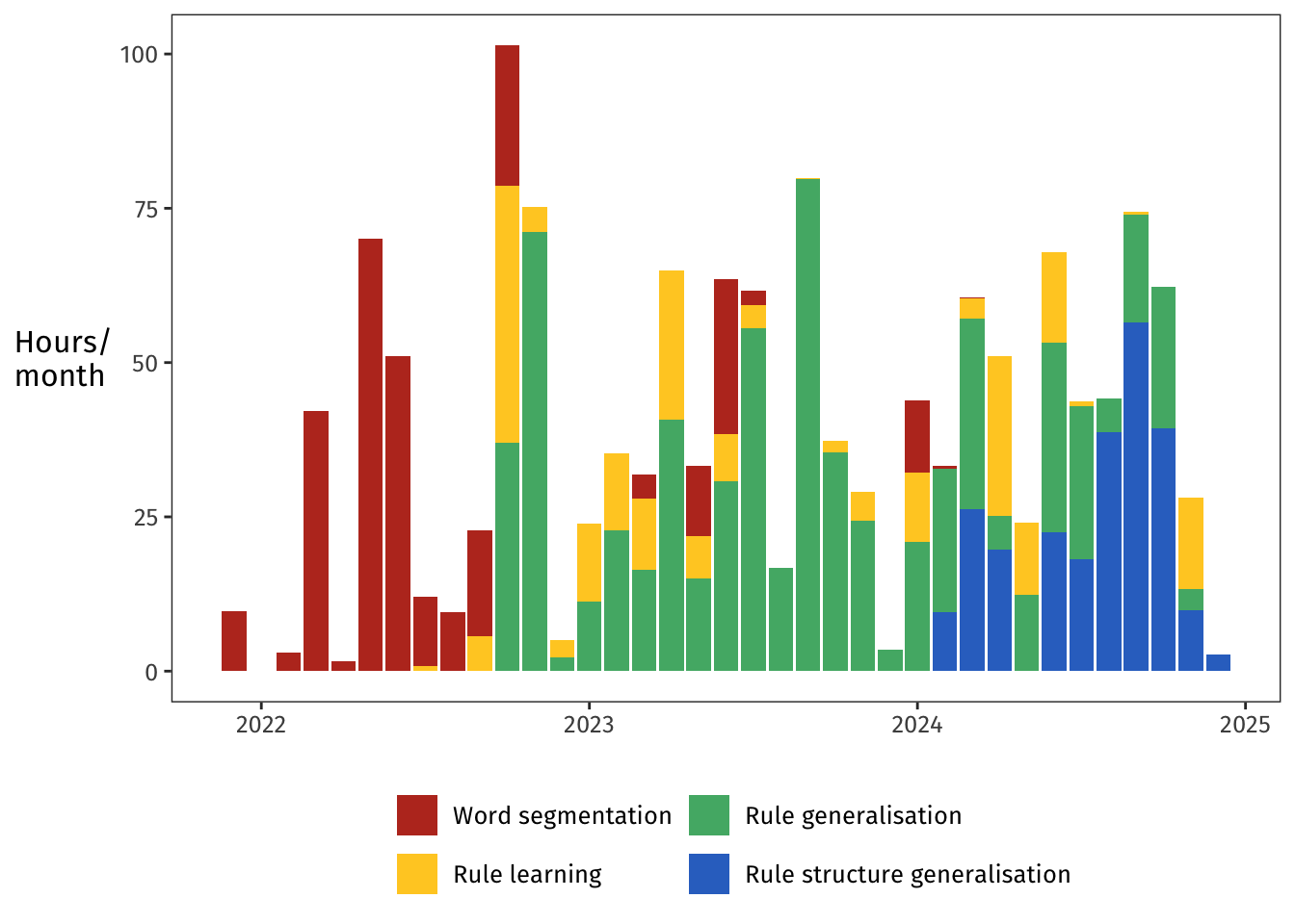
# Research projects over time
One of the plots I was most curious to generate was this next one.
```{r message = FALSE}
hrs |>
  filter(tasklabel %in% main_projs) |>
  group_by(month_idx, tasklabel, year) |>
  summarise(hrs = sum(mins)/60) |>
  mutate(tasklabel = factor(tasklabel, levels = main_projs)) |>
  ggplot(aes(x = month_idx, y = hrs, fill = tasklabel)) +
  geom_bar(stat = 'identity', position = 'stack') +
  scale_x_continuous(
    breaks = c(5, 17, 29, 41),
    labels = c(2022, 2023, 2024, 2025),
    ) +
  scale_fill_manual(values = palette_proj) +
  theme(
    legend.position = 'bottom',
    ) +
  labs(
    y = 'Hours/\nmonth',
    x = element_blank(),
    fill = element_blank(),
  ) +
  guides(
    fill=guide_legend(nrow=2),
    ) +
  NULL
```
The **Word segmentation** project (red, Chapter 2) was my first-year project, and it grew up to become [Pankratz et al., (2024)](https://onlinelibrary.wiley.com/doi/10.1111/cogs.13429).
For this project, I ran one experiment in July 2022.
The manuscript was submitted in late 2022, and the splashes of red in 2023 were the revisions following peer review.
Then in early 2024 came the final formatting checks, and then the paper was out!
The **Rule learning** project (yellow, Chapter 3), which I did together with [Aislinn Keogh](https://aislinnkeogh.github.io), is the longest-running project of the four.
We ran two experiments, one in April 2023 and one almost a year later in March 2024.
This project never got published, but it appears as a chapter in each of our PhD theses.
The **Rule generalisation** project (green, Chapter 4) consumed my time and my thinking for much of 2023 and well into 2024.
I consider it the heart of my PhD—it's the project I find the most interesting and the most compelling.
Which explains why I spent 661 hours on it!
The project did have some false starts, though.
I ran one experiment for it in October 2022, but that experiment never saw the light of day because of confounds in the design that I detected too late.
A second experiment, the one that actually appears in the thesis, was run in July 2023.
Finally, the **Rule structure generalisation** project (blue, Chapter 5) was my main focus in my final year.
For this project, I ran four experiments within three months: one in June 2024, two in August, and one in September.
Those four experiments were all pretty similar, but still, four experiments in three months is serious progress, considering I spent my entire first year on one single experiment!
Turns out a PhD does actually teach you things.
Who knew?
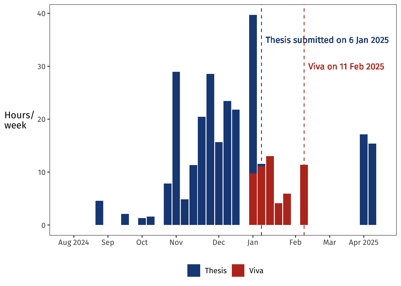
# Thesis writing and viva prep
In addition to the four content chapters, my thesis contains an introduction chapter, a general discussion chapter, and a bunch of appendices.
The time I spent planning, writing, and revising that thesis-specific material was recorded as **Thesis** time.
**Thesis** time also contains hours spent on LaTeX tomfoolery and on implementing the minor corrections after my viva.
Under **Viva** time, I counted the hours I spent designing my pre-viva talk (which is probably my favourite talk I've ever given) as well as doing more traditional prep for the viva itself.
Here I'll plug Nathan Ryder's [Viva Survivors](http://viva-survivors.com) web site and workshop, and especially the [7776 Mini-Vivas resource](http://viva-survivors.com/2018/11/new-resource-7776-mini-vivas/).
Doing a mock viva using that resource was the most useful part of my prep by a mile.
```{r}
hrs |>
  filter(tasklabel %in% c('Thesis', 'Viva')) |>
  group_by(tasklabel) |>
  summarise(hrs = round(sum(mins)/60)) |>
  knitr::kable()
```
All in all, I spent 235 hours on thesis-specific tasks and 55 hours creating the pre-viva talk and preparing for the viva itself.
Here's how those hours played out over time:
```{r message = FALSE}
hrs |>
  filter(tasklabel %in% c('Thesis', 'Viva')) |>
  group_by(week_idx, tasklabel, year) |>
  summarise(hrs = sum(mins)/60) |>
  ggplot(aes(x = week_idx, y = hrs, fill = tasklabel)) +
  geom_vline(xintercept = 175, colour = palette_exam[1], linetype = 'dashed') +
  geom_text(x = 175.5, y = 35, label = 'Thesis submitted on 6 Jan 2025', hjust = 0, family = 'Fira Sans', colour = palette_exam[1]) +
  geom_vline(xintercept = 180, colour = palette_exam[2], linetype = 'dashed') +
  geom_text(x = 180.5, y = 30, label = 'Viva on 11 Feb 2025', hjust = 0, family = 'Fira Sans', colour = palette_exam[2]) +
  geom_bar(stat = 'identity', position = 'stack') +
  scale_x_continuous(
    breaks = c(153, 157, 161, 165, 170, 174, 179, 183, 187),
    labels = c('Aug 2024', 'Sep', 'Oct', 'Nov', 'Dec', 'Jan', 'Feb', 'Mar', 'Apr 2025'),
    limits = c(152, 189)
    ) +
  scale_fill_manual(values = palette_exam) +
  scale_colour_manual(values = palette_exam) +
  theme(
    legend.position = 'bottom',
  ) +
  labs(
    y = 'Hours/\nweek',
    x = element_blank(),
    fill = element_blank(),
  ) +
  NULL
```
I spent most of November and December writing.
After a week off during the holidays, the thesis was ready to submit by early January, and then I turned immediately to preparing for the viva in mid-February.
Following the viva, I took a month to prepare for a job interview, and then in April I picked up the thesis again and worked on my corrections for two relaxed weeks.
Those corrections were submitted on 9 April and approved on 15 April, and now, 242,516 minutes later, I can call myself Doctor 😊
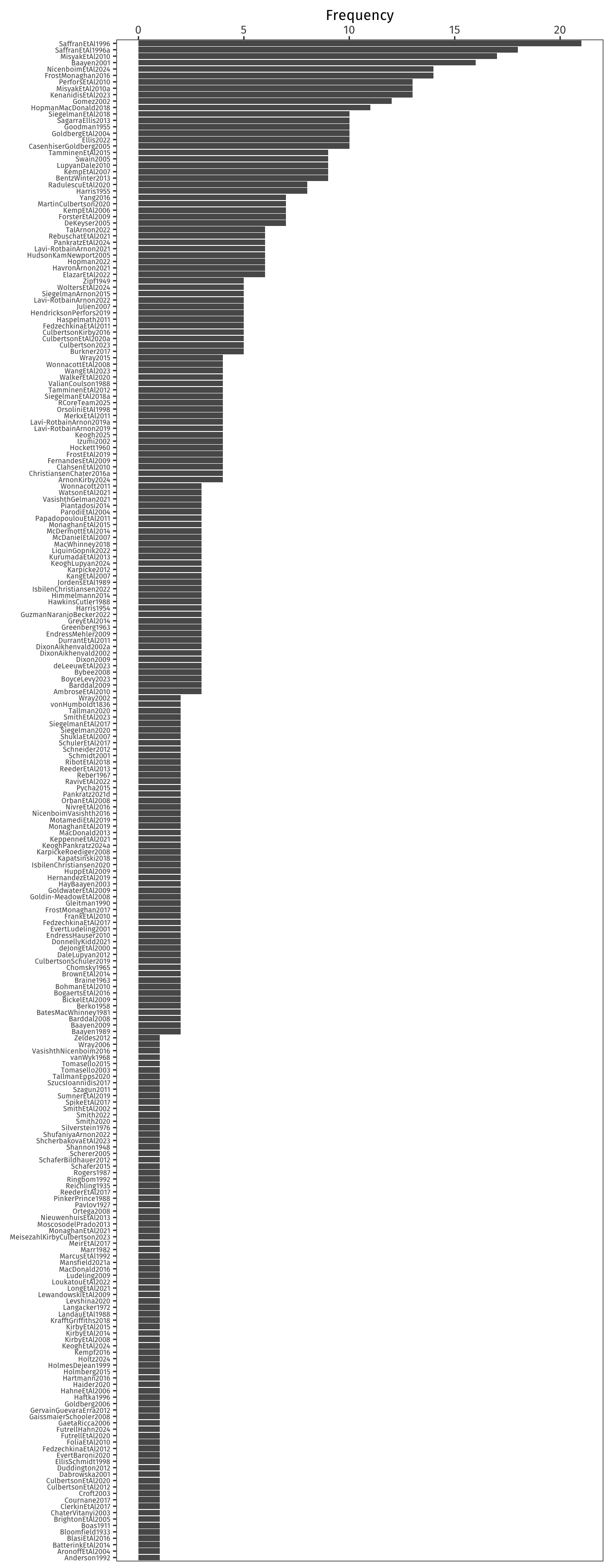
# Epilogue: Citation frequencies
As a cherry on top, I wanted to look at how often I cited each piece of literature.
Each citation is itemised in the `.bcf` file produced by biblatex.
And, surprise surprise, Zipf appears both in name and in rank/frequency law:
```{r fig.height = 18}
bcf <- xml2::read_xml('data/output.bcf')
citekeys <- xml2::xml_text(xml2::xml_find_all(bcf, ".//bcf:citekey"))
refs_freqdist <- as.data.frame(table(citekeys)) %>%
  arrange(Freq) %>%
  mutate(citekeys = factor(citekeys, levels = citekeys))

refs_freqdist %>%
  ggplot(aes(x = Freq, y = citekeys)) +
  geom_bar(stat = 'identity') +
  labs(
    y = element_blank(),
    x = 'Frequency'
    ) +
  theme(axis.text.y = element_text(size=6)) +
  scale_x_continuous(position = 'top') +
  NULL
```
(Zipf, 1949 shows up in Rank 49 with a frequency of 5.)
Appropriately, considering my PhD was about how distributional statistics affect language learning, my top five sources are:
1. Saffran, J. R., Aslin, R. N., & Newport, E. L. (1996). Statistical learning by 8-month-old infants. *Science*, 274(5294), 1926–1928. <https://doi.org/10.1126/science.274.5294.1926>
2. Saffran, J. R., Newport, E. L., & Aslin, R. N. (1996). Word segmentation: The role of distributional cues. *Journal of Memory and Language*, 35(4), 606–621. <https://doi.org/10.1006/jmla.1996.0032>
3. Misyak, J. B., Christiansen, M. H., & Tomblin, J. B. (2010). On-line individual differences in statistical learning predict language processing. *Frontiers in Psychology*, 1. <https://doi.org/10.3389/fpsyg.2010.00031>
4. Baayen, R. H. (2001). *Word frequency distributions*. Kluwer Academic Publishers.
5. Frost, R. L. A., & Monaghan, P. (2016). Simultaneous segmentation and generalisation of non-adjacent dependencies from continuous speech. *Cognition*, 147, 70–74. <https://doi.org/10.1016/j.cognition.2015.11.010>
Many processes lead to Zipfian distributions, indeed...
# Session info
```{r}
#| code-fold: false
sessionInfo()
```