Getting set up
Download files
I’ve created a pre-loaded directory structure for this workshop that you can download. (If you’re having internet issues, ask me for the version on USB.)
- Right-click on this link and download the zip file (3.1 MB).
- Unzip it and relocate the directory to wherever you want on your computer.
- To open the R project, click on the file
bayes_workshop.Rproj(you might not see the.Rprojpart—then just click on the thing that saysbayes_workshop). This will open the R project within RStudio; you’ll be able to tell you’re in the R project because at the top right of your RStudio window, you’ll see its name:

- In the Files pane at the bottom right of RStudio, click on
code/and open the file calledworkshop.Rmd.
R projects can be very helpful for creating reproducible analyses. For one, they let you set RStudio’s working directory to the project directory (i.e., the directory where the .Rproj file lives), and this makes reading in data that also lives within the project directory very easy.
You can see this at work in the R notebook I’ve prepared.
Open workshop.Rmd
workshop.Rmd is where you’ll build up the code to fit your Bayesian model.
First up, make sure that the code that’s already in workshop.Rmd runs as it should. Execute all the code chunks in this file.
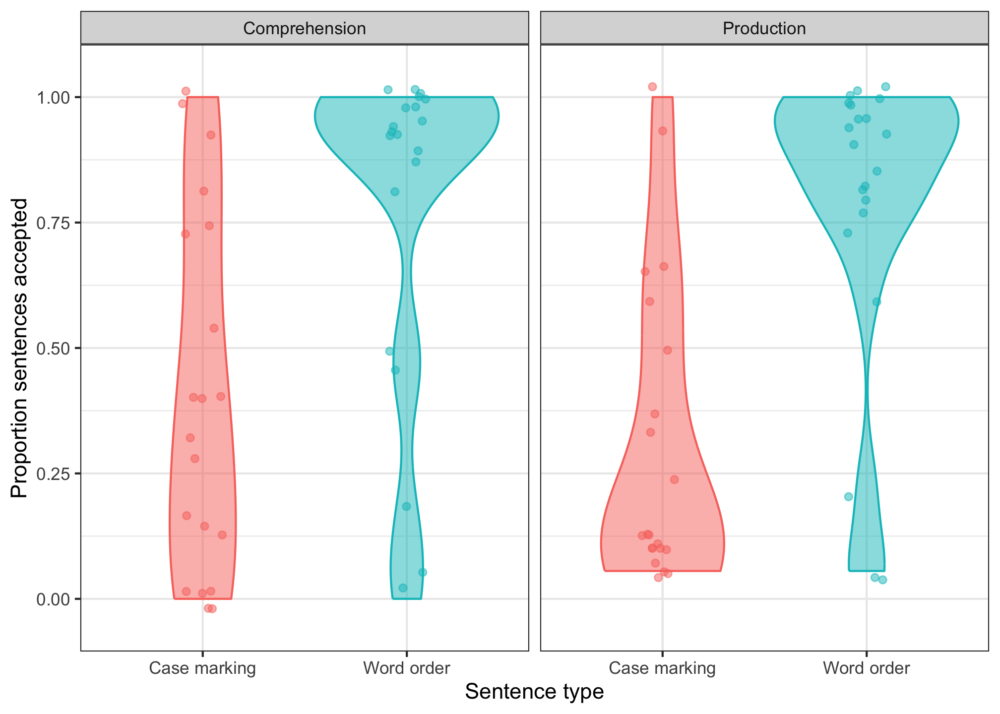
If everything is running correctly, you should see (1) no errors, (2) six lines of data, and (3) a plot that looks like this:
If you do, then you’re good to go! If not, let me know and we can troubleshoot.
The data we’ll use
This data is a subset of the full dataset from a recent study run by Aislinn Keogh and Elizabeth Pankratz. We wanted to know whether the type of experimental task that participants do (a comprehension task vs. a production task) can affect whether participants learn a word order grammar or a case marking grammar for an artificial language where both analyses are possible. (For more detail on the project, come see our virtual poster at CogSci this summer and stay tuned for our preprint 😉)
We’ll look at data from this experiment’s judgement phase, where participants are shown novel sentences that are constructed using either the word-order grammar or the case-marking grammar—sentences that are not compatible with both analyses. If participants learned one grammar, they should accept sentences constructed with that grammar and reject the others. In particular, we wanted to know whether participants in the production group would be more likely to accept case-marking sentences than participants in the comprehension group.
The plot you see in workshop.Rmd shows that this doesn’t seem to be the case—in fact, production participants reject case-marking sentences even more than comprehension participants do!
Prepare the data
We are going to use \(\pm\) 0.5 sum coding for the condition variable (comprehension as –0.5; production as +0.5) and for the sentence type variable (case marking as –0.5; word order as +0.5). Our hypothesis concerns the interaction between these predictors, so we’ll include an interaction term as well. An interaction is the product of the two interacting variables, and we’ll scale that by two so that the interaction also takes the values \(\pm\) 0.5.
To set up the predictors we’ll use, copy and run the following code in your R notebook:
acc <- acc %>%
  mutate(
    cond = ifelse(condition == 'Comprehension', -0.5, 0.5),
    sent = ifelse(sentence_type == 'case_marking', -0.5, 0.5),
    condsent = cond * sent * 2
  )
(There are, of course, ways to set contrasts without creating whole new columns, e.g., using contr.sum(2)/2, but I like this way because it’s super explicit about what information the model’s going to use.)
Next, let’s have a look at how to model this data using brms.